Week 9 Progress: Feature Engineering
- Creating models to test our data and predict values
- Also Redoing our Engineered features in accordance to our new "Response Variable" and the addition of the new variable "Temperature"
EDA (Secondary)
- Principal Component Analysis
Figure 1: 2D biplot of our new Dataset.
The 2D Biplot above is of normalized data with respect to the principle components (PC1 and PC2) and the variables Billed, Generated, Sent out and Tmp2m_C_ which represents the power that is generated from renewable energy which in this case is solar energy, wind energy and BESS. It can be seen that Tmp2m_C_ has a very high positive correlation on PC1. Billed can be said to have least influence on PC1 and PC2. Due to its weak correlation, billed may require feature engineering to improve forecasting accuracy. Meanwhile, there is very little separation between the Generated and Sent out variables due to the difference from line loss.
Figure 2: new correlation map
The heatmap above shows the pairwise relationships between the four variables—GENERATED, SENT_OUT, BILLED, and Tmp2m_C_—are displayed in this correlation heatmap. The Pearson correlation coefficient, which measures the strength and direction of a pair of variables' linear relationship, is displayed in each cell of the matrix. Since every variable has a perfect correlation with itself, all of the diagonal values are 1. Stronger positive correlations are indicated by darker blue hues in the heatmap, which shows the correlation's magnitude. All four variables are positively and strongly associated, according to this heatmap, GENERATED, SENT_OUT, and BILLED are close correlated. This suggests that energy flows and is tracked consistently throughout the generation, distribution, and billing operations. Tmp2m_C_'s somewhat lower correlation raises the possibility that it has a secondary function or is more variable.
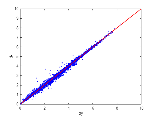
Figure 3: New PCA
This shows that the variables are highly redundant which may be due to the three variables Billed, Generated and Sent out as they are only separated by small losses. Meanwhile, the dy-dx plot shows that the distance in the reduced dimensional space remains very close to that of the original.
After carrying out CCA, the above dy-dx plot was made. The plot shows that the points cluster well around the diagonal line, indicating that CCA has effectively preserved the pairwise distances.
Modelling for our Original Features
- The ARIMA - Integrated & Moving Average

Figure 5: AIMA modelling
The figure shows the best model (ARIMA) trained to give a higher accuracy performance. Though there are some minor over and under sizing it can be taken care of by having a complex structure to refine its predictions. The RSME value is also at its lowest value (close to zero) showing less losses.
- SARIMA - Seasonal Autoregressive Integrated & Moving Average

Figure 6: SARIMA modelling
The graphs shows an offset, that maybe caused due to some NaN values. This maybe be corrected through more refinements in the datasets or having the coding structure be more complex so the training model can learn the patterns more efficiently.
- LSTM - Long Short Term Memory

Figure 7: LSTM modelling
In this representation, the ideal dream is achieved, however, the system is over performing the predicted values which is good but causes unnecessary power loss or wastage if produced and followed by this model. Maybe, through more epochs or iterations the system will behave in a manner suitable to deploy into power utility.
- CNN - Convolutionary Neural Networks

Figure 8: CNN modelling
For this figure it can be seen that the model is able to somewhat predict the varying data sets of the actual data, however is it having a difficulties in under predicting. This could be due to the complexity of the code structure, whereby the number of iterations isn't enough for the model to train itself to predict more better accurate R^2 value. As for the measuring metrics it is somewhat possible to use the metrics value, however, as a model it should be having a RMSE value closer to zero.
Modelling for our Original features together with the Engineered Features
- The ARIMA - Autoregressive Integrated & Moving Average

Figure 9: ARIMA modelling
The figure shows the best model (ARIMA) trained to give a higher accuracy performance. Though there are some minor over and under sizing it can be taken care of by having a complex structure to refine its predictions. The RSME value is also at its high time lowest value (close to zero) which shows a great adaptability and less errors and losses.
- SARIMA - Seasonal Autoregressive Integrated & Moving Average

Figure 10: SARIMA modelling
In the figure above, the predicted values can be seen having a offset that maybe caused due to some NaN values. This maybe be corrected through more refinements in the datasets or having the coding structure be more complex so the training model can learn the patterns more efficiently.
- LSTM - Long Short Term Memory

Figure 11: LSTM modelling
In the graphical representation, it can be said if more epochs were added together with more batch size the model would have a higher accuracy in predicting the actual datasets or having a more precise values.
- CNN - Convolutionary Neural Networks

Figure 12: CNN modelling
For the figure above the reason for a miss prediction could be due to less layers or complexity in the coding for the model to train more and understand the features to able to produce a more reliable predicted data points. AS for the measuring metrics it could also be due to the inefficient training to accurately predict and have a more lesser RMSE value.
Remark
So far 4 models have been trained and tested, ARIMA, SARIMA, LSTM, CNN and Linear Regression. After inspecting the results obtained, the ARIMA and Linear Regression model produced the best results as the RMSE, MAE and MAPE values more desirable. However, the next tasks will include improving all the models particularly the LSTM and CNN by adding more layers and complexity to the model in order to increase the performance of the models. Also, at least two other models will be researched on in the coming weeks and trained, allowing a wider range possible models to choose from.


Comments
Post a Comment